Pathtracer

• Overview
• Ray Generation and Intersection
• Bounding Volume Hierarchies
• Direct Illumination
• Global Illumination
• Adaptive Sampling
• Reflective and Refractive BSDFs
• Microfacet BRDF
• Thin Lens and Autofocus

Overview

This project was done for CS184 Computer Graphics & Imaging at UC Berkeley, taught by Professor Ren Ng. In this project, I implemented the core functionality of a physically-based renderer and the rendering equation.

In path tracing, rays are traced from the camera through each pixel of an image into a three-dimensional scene, where they encounter different surfaces.

At each intersection with a surface, the outgoing light towards the camera is computed using the total incoming light and the Bidirectional Scattering Function (BSDF) of that surface. The incoming light that reaches that point is found by tracing the ray recursively back through the scene, and accumulating the light reflected or transmitted by different surfaces (or light sources) at each subsequent intersection with a surface.

By integrating over all the light arriving at a point and scaling it by the BSDF, we can determine the final amount of radiance towards the camera and compute the color of the pixel.

This process is repeated for every pixel to form an entire image.

Ray Generation and Intersection

Imagine a virtual camera looking at scene; each pixel of the final image has a corresponding location on that virtual camera sensor.

First, we convert the pixel’s location from image space to camera space:

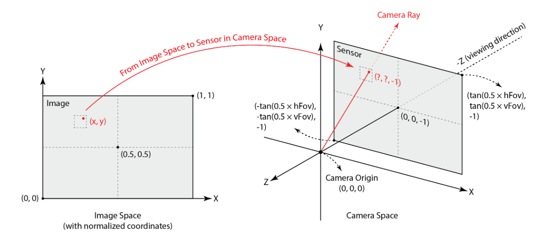
Then, we can define a ray that starts at the camera’s origin and goes through the location of that pixel on the virtual camera sensor, like a little hole in a mesh screendoor. Note that rays should exist in world space–the world of the scene.

Since pixels are specified by the coordinates just one of their corners, we generate a bunch of rays over the unit square of each pixel by random sampling (each ray has an ever-so-slightly different direction).

For each ray, we need to check for an intersection with a surface in the scene. We can see if a ray and a triangle intersect using the Möller-Trumbore algorithm:

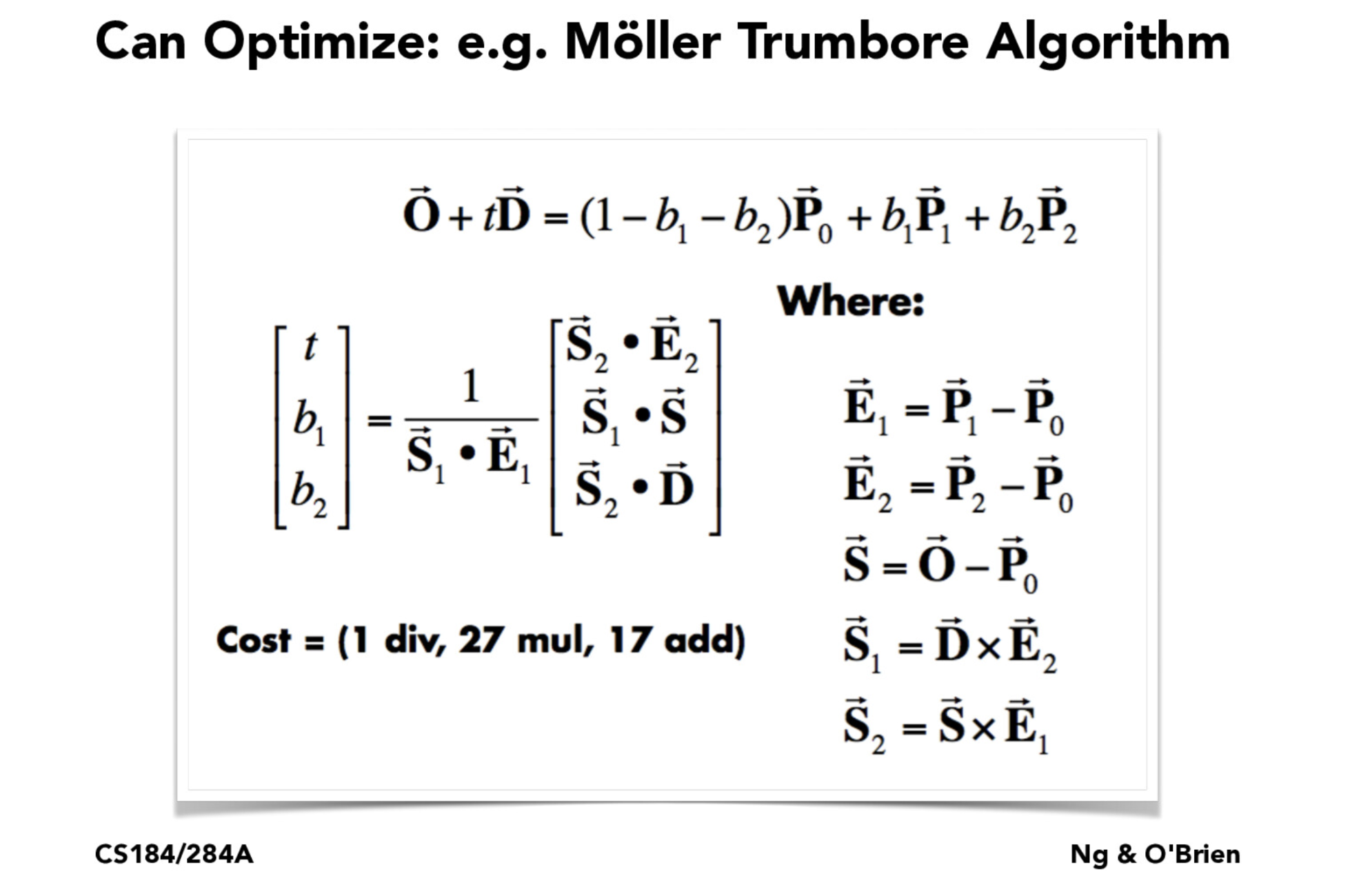
This algorithm takes a ray with origin O and direction D and tests for its intersection with a triangle with vertices P₀ , P₁ , and P₂ . If the barycentric coordinates b₁ , b₂ , and 1 - b₁ - b₂ specify a point within the triangle, then there is an intersection.

However, testing against every triangle in a scene for an intersection is costly and inefficient, so I accelerate this process by constructing a bounding volume hierarchy for the scene.

Bounding Volume Hierarchies

A bounding volume hierarchy (BVH) is a tree in which each node is the bounding box of a collection of primitives in a mesh, and the leaves are the individual primitives themselves (triangles). Instead of testing for an intersection with every primitive in a mesh, we can check for intersection with bounding boxes, and only check for intersection against individual primitives when we hit a leaf.

At each layer of BVH construction, I choose to split the primitives into left or right branches of the BVH using their average centroid as the split point.

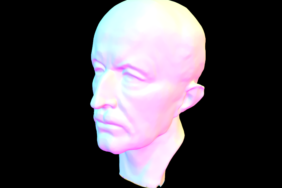
The BVH is constructed recursively. The intersection test for each ray improves from linear to logarithmic time, so now we can quickly generate images of complicated meshes with thousands of triangles:

Direct Illumination

First, I implemented direct illumination. A point on a surface is visible if any rays reflected from the surface directly intersect a light source.

For Lambertian surfaces, reflection is equally diffuse in all directions around the point of intersection. Upon finding an intersection with a surface, we can sample the direction of reflected rays using uniform hemisphere sampling, where we choose a random direction within a hemisphere centered around the surface normal at the point of intersection.

We generate a ray that starts at the point of intersection and trace it in the direction to check if it intersects a light source. Using the amount of incoming light from the source, we can compute the outgoing light using the reflectance equation:

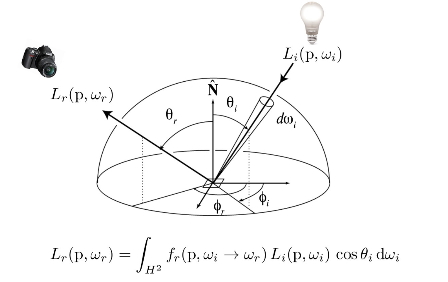
The total outgoing emission at point p in the direction wr is Lr(p, wr), and the integral of the total emission coming from every outgoing direction wi is over a hemisphere H².

Li(p, wi) is the emission from a light source that a ray starting at p with direction wi encounters, fr(p, wi -> wr) is the evaluation of the BSDF at point p of a ray being reflected from wi to wr towards the camera, and cos(θi) is used to attenuate the amount of light coming in from an angle.

In practice, we approximate this with a Monte Carlo estimator with N samples and the probability distribution function (for a hemisphere, this is 1/2π):

However, the renders we get back are noisy because many sampled rays never reach a light source at all. While this image would eventually converge, we would need way too many samples. Additionally, sampling uniformly on a hemisphere is unable to practically sample point light sources.

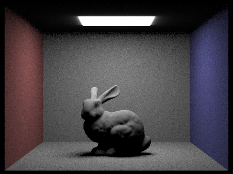
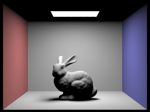
A better solution is to use importance sampling of lights, where we sample rays in the directions of our scene lights instead of randomly over a hemisphere. A point is directly illuminated only if the rays do not intersect any other surface before reaching the light source.

We perform this sampling process for every light source in the scene and sum together the radiance contribution from each light.

Now, the renders are far less noisy because they take far fewer samples to converge.

Global Illumination

In the real world, objects are illuminated not only by direct light sources, but also indirectly by light reflected or transmitted by other objects in the environment.

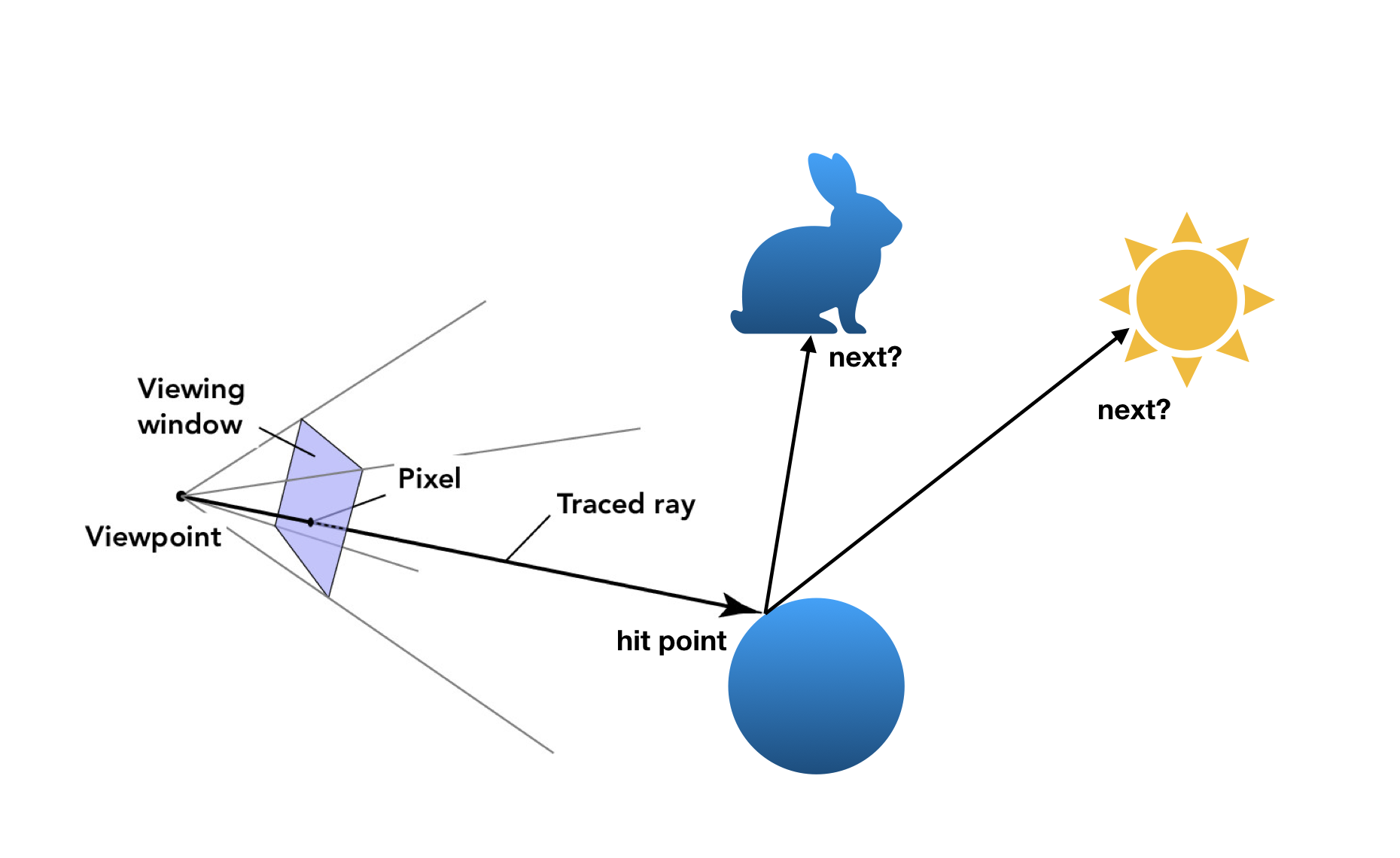
To simulate this physical process, I recursively trace each ray back through the scene until it either intersects a light source or we choose to terminate the ray. We can terminate the ray based on Russian Roulette, an unbiased method of random termination, as well as by setting a max number of bounces.

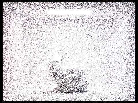
The contribution of later bounces to the final pixel radiance decreases exponentially because it should be attenuated by the BSDF at each surface along the way. At first, I forgot to consider that and the renders came out far too bright. An example of a buggy render:

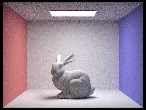
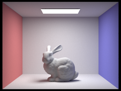
Upon fixing this bug, I now have global illumination. We can see some of the color bleeding from the red and blue walls on the right and left sides of the model:

One way to reduce the noise of the images is to increase the number of rays sampled per pixel. At 1024 rays per pixel, the noise is almost impossible to notice.

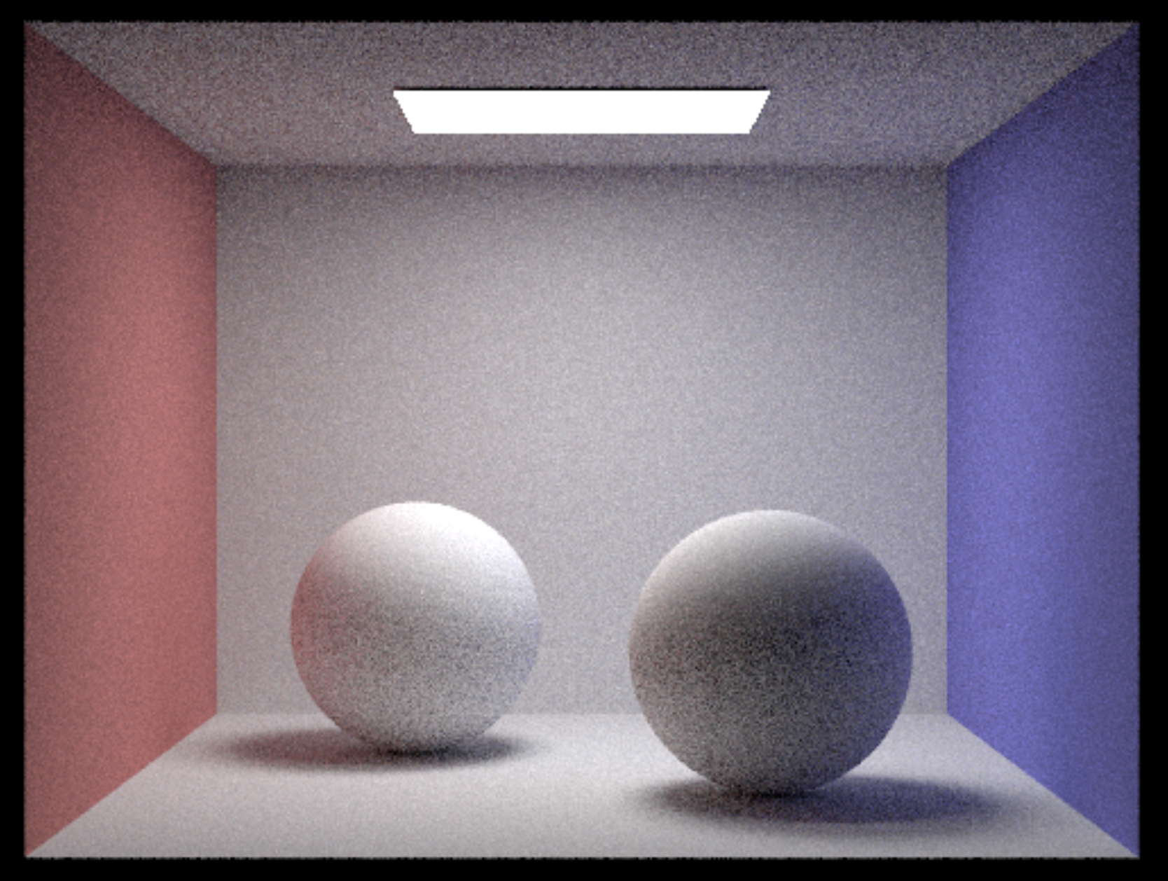
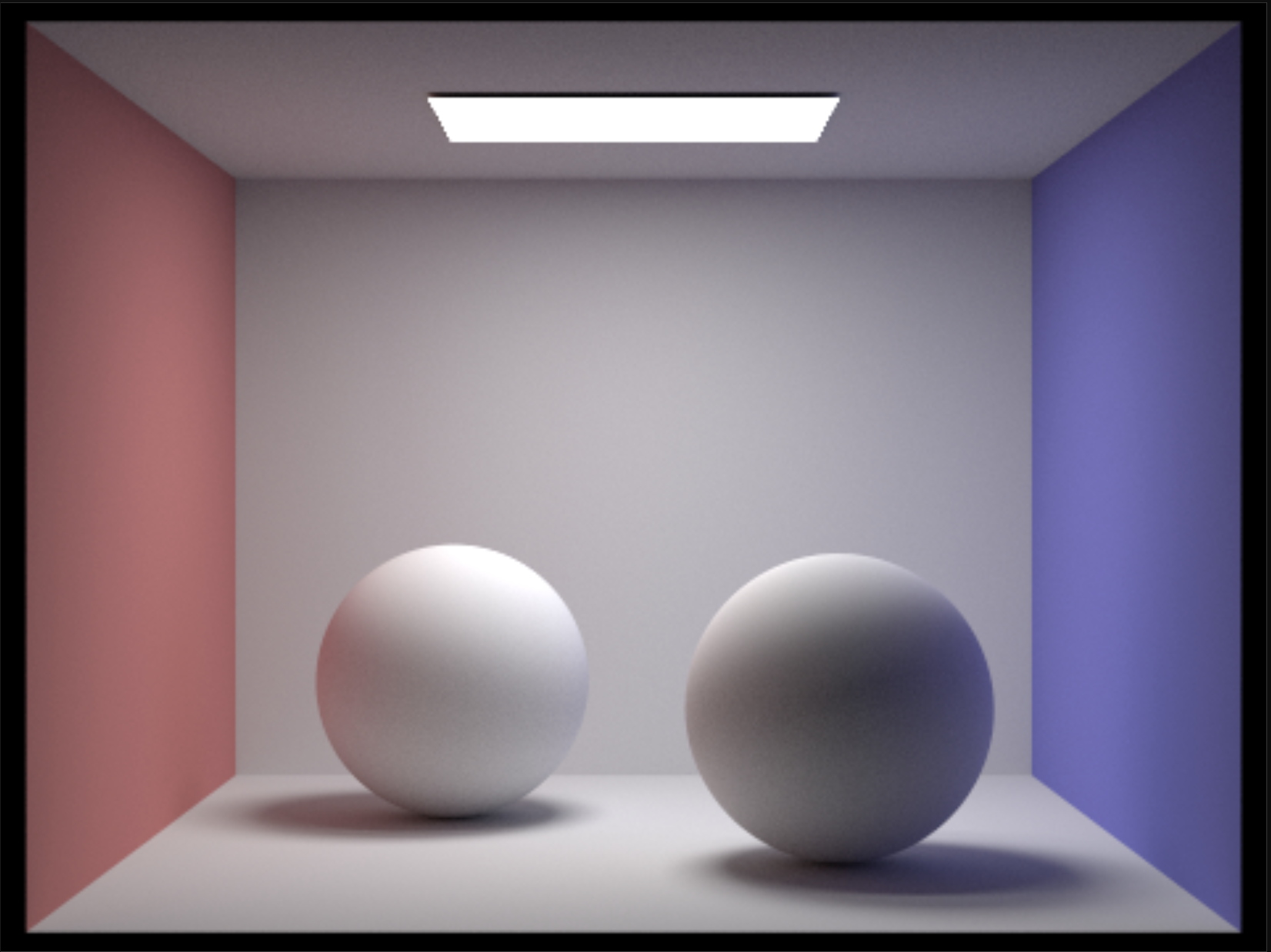
However, taking many samples is a slow and computationally expensive process. We can speed up our renders with adaptive sampling.

Adaptive Sampling

With adaptive sampling, we check if a pixel’s value has converged early as we trace rays through it, and stop sampling if it has.

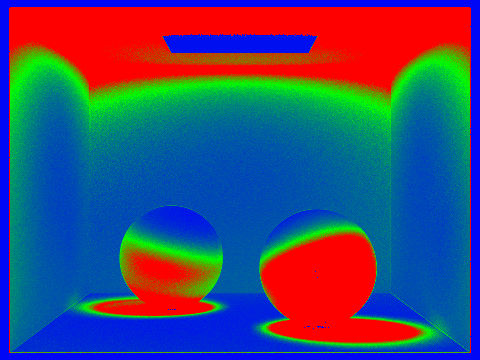
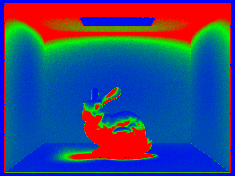
We can check a pixel’s convergence after each batch of n samples to see if it’s within a 95% confidence interval. Areas of the scene that are shadowed or not directly illuminated take longer to converge. Below are images depicting sample rates for Cornell box spheres and bunny: red indicates that we took more samples to converge, while blue and green indicate that the pixel value converged quickly and we stopped sampling earlier.

And finally, here is the bunny render, using 1024 samples:

Reflective and Refractive BSDFs

So far, I have only modeled Lamberian materials with diffuse reflection. To simulate other materials like metal or glass, I implement reflective and refractive BSDFs.

For a perfectly reflective mirror-like surface, the angle between the incoming incident ray and the surface normal is equal to the angle between the surface normal and the outgoing ray.

For refractive surfaces, the direction of the transmitted ray is modeled by Snell’s Law. When modeling refraction, we also consider the edge case of total internal reflection, when a light ray is internally reflected instead of crossing the boundary between two mediums.

We need a minimum ray depth of 2 to have reflections from not only direct light sources but also the surrounding environment:

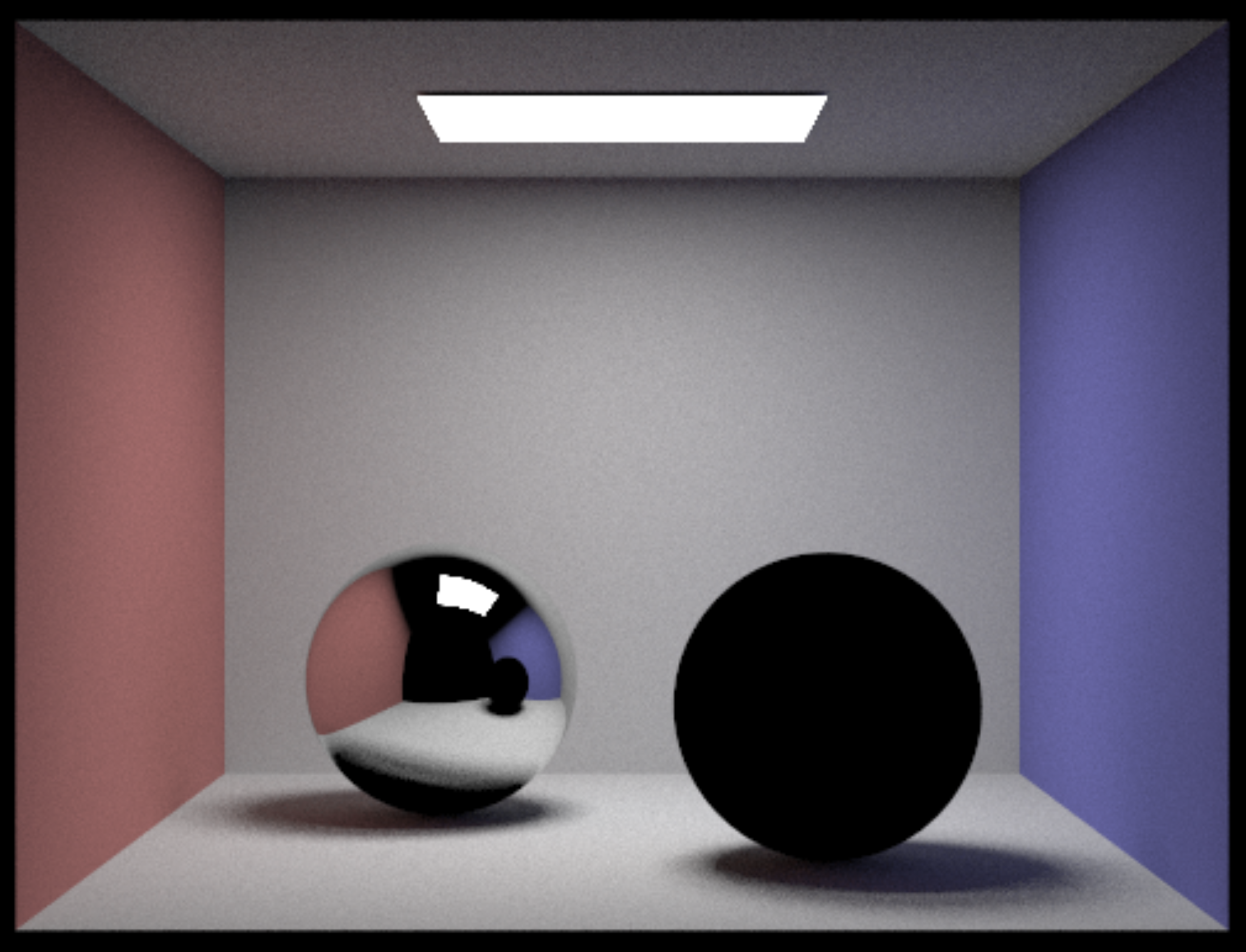
We need a minimum ray depth of 3 to have refraction (the light must first enter the sphere and also exit the sphere before reaching the environment). Note the caustic effect in the bottom right corner, a sign of refraction. At a ray depth of 4, light refracted through the glass sphere on the right can be reflected off the mirror sphere on the left, and we can see its reflection as well.

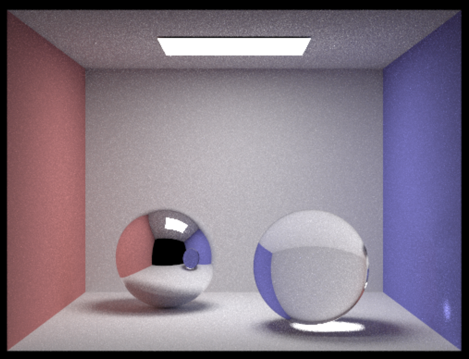
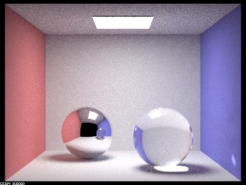
The sphere on the right is purely refractive right now. More realistic glass exhibits both refraction and reflection. The ratio of reflection to refraction is modeled by the Fresnel equations in physics, but I model this with Shlick’s approximation to make it easier to evaluate. Now, we can see the reflection of the ceiling light on the glass ball on the right as well.

Microfacet BRDF

We can also model microfacet materials–those with a rough reflective surface such as brushed metal—with a microfacet BRDF. This implementation closely follows the method outlined in this article. Specifically, we use this equation to evaluate the BRDF:

Where F is the fresnel term, G the shadow-masking term, D the normal distribution function, n the normal at the macro level, and h the half-vector (the normal at the microsurface).

For D(h), I implement the Beckmann distribution, which is more suited to microfacet materials than the Gaussian distribution:

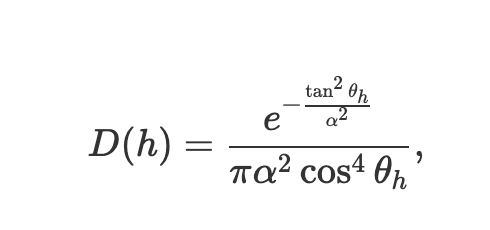
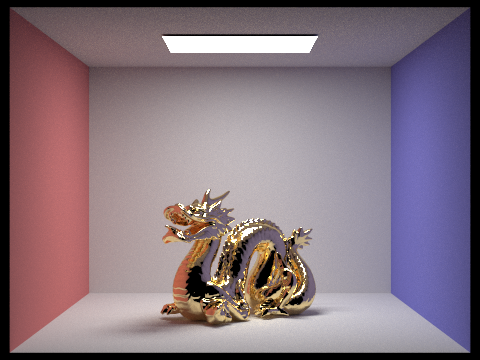
Here, α represents the albedo, or the reflectance of a material. We use this to control the glossiness or reflectance of a material. Below is a render of a dragon with a gold material and albedo α = 0.05.

Thin Lens and Autofocus

Finally, I can extend the path tracer’s virtual camera, which follows an ideal pinhole model, to use a thin lens instead. With a pinhole model, everything is in perfect focus. However, lenses in real cameras and human eyes have a finite aperture and focal length.

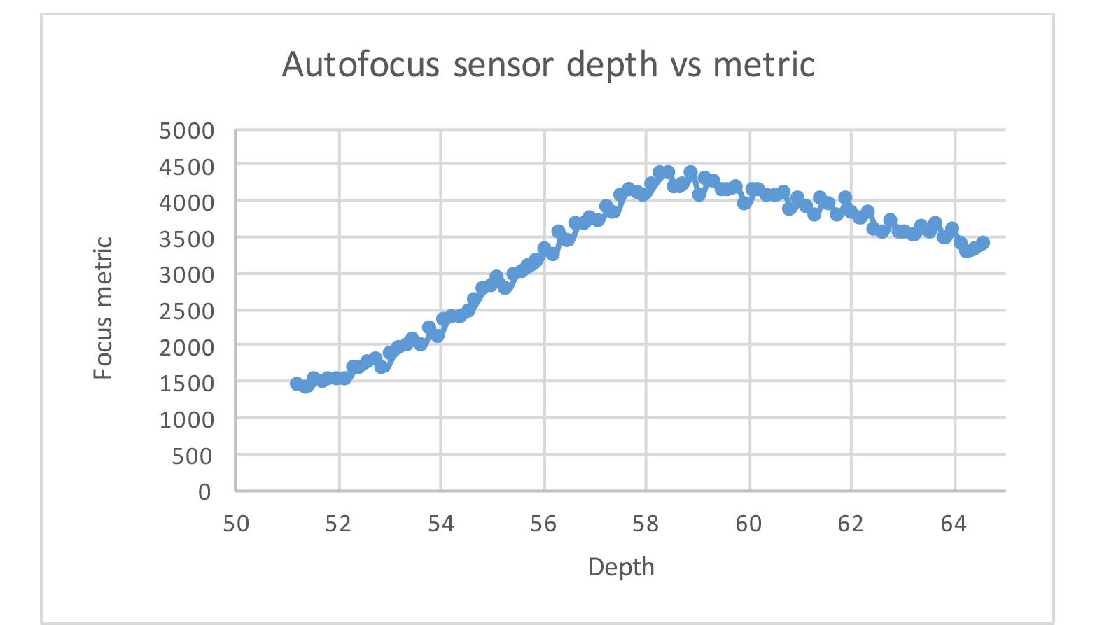
I first create lens elements that refract the rays first in accordance with Snell’s Law, to create depth of field. Next, I implement contrast-based autofocus with a focus metric based on the sum of the variances of an image patch to focus on. By stepping through the depths between my infinity-focus and near-focus positions, I can find the location of the virtual camera sensor that maximizes the amount of contrast in the region I want to be in focus.

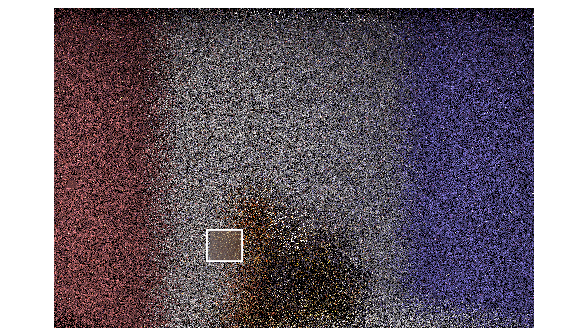
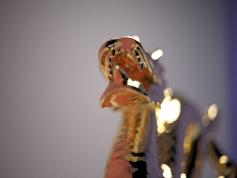
Using a double Gauss lens model, the most common type of camera lens, I can focus on this region of the dragon’s head.