Cloth Simulation

Under construction!

• Overview
• Mass-Spring System
• Numerical Integration
• Collision Handling
• Self-Collisions
• GLSL Shaders
  • Diffuse and Blinn-Phong Shading
  • Texture Mapping
  • Displacement and Bump Mapping
  • Environment Reflection Mapping

Overview

Cloth can be simulated with a 2D grid of point masses connected by springs, as outlined in this 1995 SIGGRAPH paper. The motion of each mass is governed by the net force from external forces (e.g. gravity) and internal spring forces. The position of each mass at any point in time can be found using the laws of motion and numerical integration techniques.

Here, I implement this mass-spring system and accelerate neighbor detection and collision handling with spatial hashing. I also implement several GLSL shaders to texture the cloth with different effects.

Mass-Spring System

Our model for the cloth is an m x n grid of identical masses connected by massless springs. There are 3 different types of spring constraints:

1. Structural constraints exist between a mass [i, j] and masses [i + 1, j] and [i, j + 1]. They help define the topology of the cloth and simulate “stretching” stresses on the cloth.
2. Shearing constraints exist between a mass [i, j] and masses [i - 1, j - 1] and [i - 1, j + 1]. They help prevent excessive shearing deformation and prevent the grid from collapsing entirely onto one side.
3. Bending constraints exist between a mass [i, j] and masses [i + 2, j] and [i, j + 2]. They simulate smooth “bending” on the cloth and prevent the grid from folding perfectly onto itself like an infinitely thin sheet of paper.

Structural and bending constraints

Shearing constraints

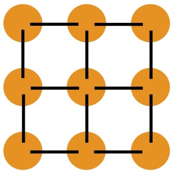
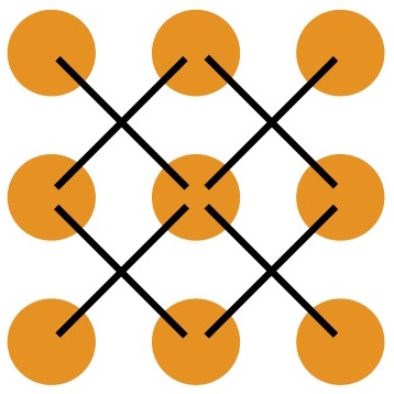
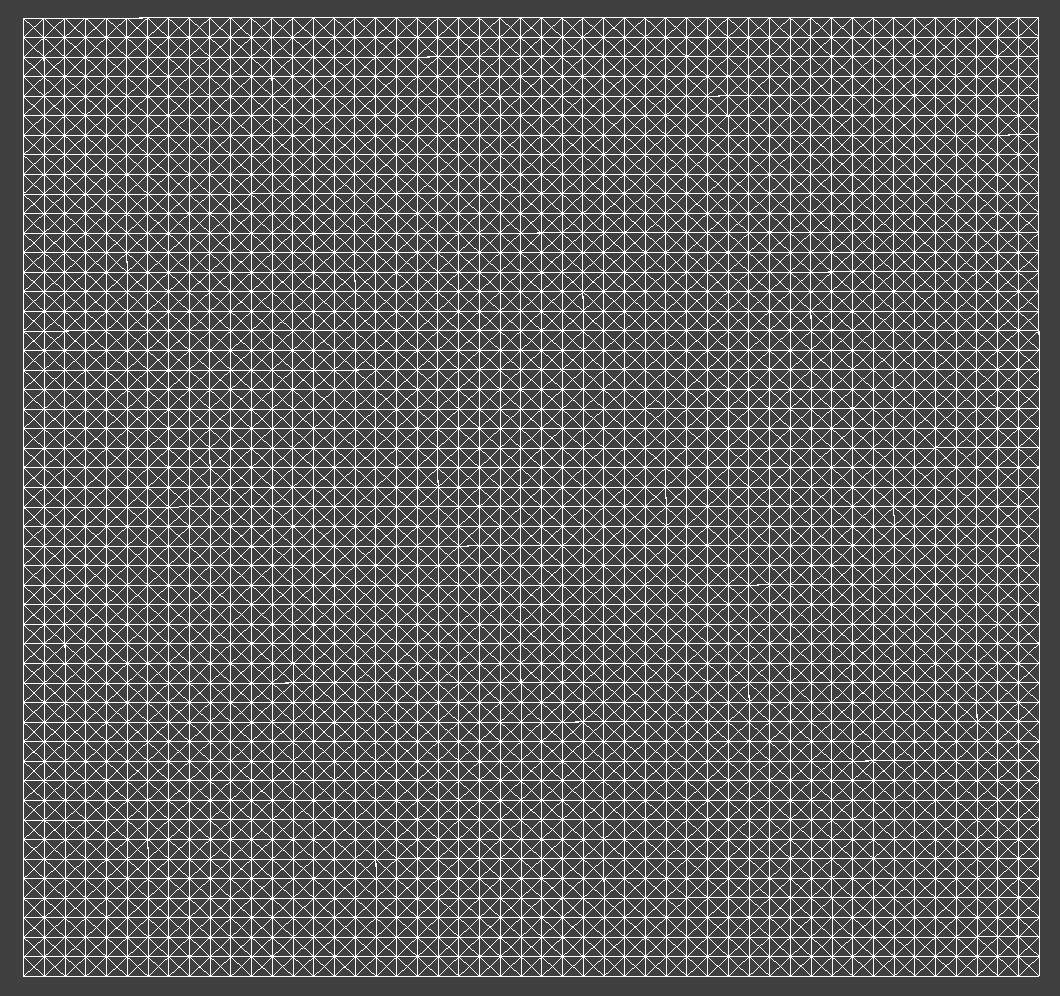
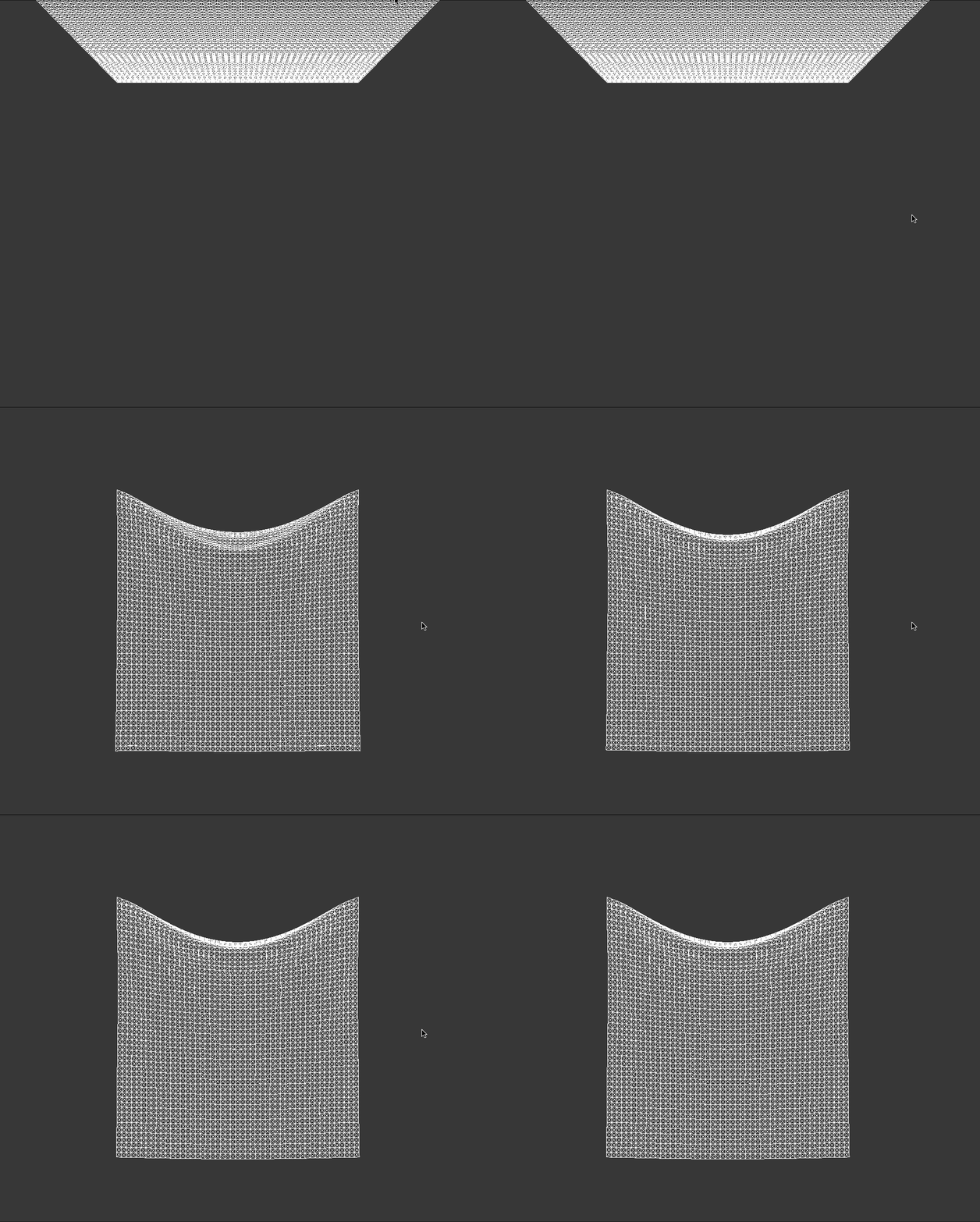
The grid with all the spring constraints between point masses set up is shown below:

Numerical Integration

The total force acting on a mass at any instant can be found by first applying any external forces and then the forces from the spring constraints. I do this by looping over all the springs and calculating the force a spring exerts on the masses at either end using Hooke’s Law:

where \(k_s\) is the spring constant, \(p_a\) and \(p_b\) are the positions of the two end masses a and b respectively, and \(l\) is the spring’s rest length. For flexion constraints, I also scale the force by 0.2 to keep them weaker than structural or shearing constraints.

Using the net force on each mass and numerical integration, I can find the change in each mass’s position at every time step \(dt\). Here, I use Verlet Integration. Given a particle position \(x_t\), its current velocity \(v_t\), and its acceleration \(a_t\), we calculate the next position \(x_{t + dt}\) as:

We find \(a_t\) by diving the net force by the mass and can approximate \(v_tdt\) as \(x_t – x_{t - dt}\):

Finally, we introduce a damping term \(d\) to simulate energy loss over time from friction.

Additionally, the positions were constrained so that the spring was never elongated by more than 10%. If it exceeds 10%, I adjust the positions of the masses to satisfy the constraint. The adjustment is shared equally between two masses unless one of them is pinned, in which case the entire adjustment goes to the unpinned mass.

Collision Handling

We can simulate collisions with external objects such as a sphere or plane. In either case, if I detect that the location of the mass passes through the surface of the geometry, I “bump” it back up to the surface of the object.

Specifically, for a sphere we find a correction vector that goes from the sphere’s origin to the position of the point mass. For a plane, the correction vector goes from the mass’s last position to a point where the mass should have intersected from the plane if it had traveled from its current position in a straight line to the surface of the plane.

We apply a \((1 - f)\) scaling factor to the correction vector to account for loss of energy from friction.

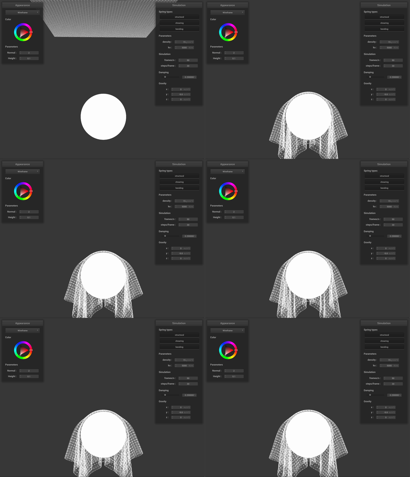
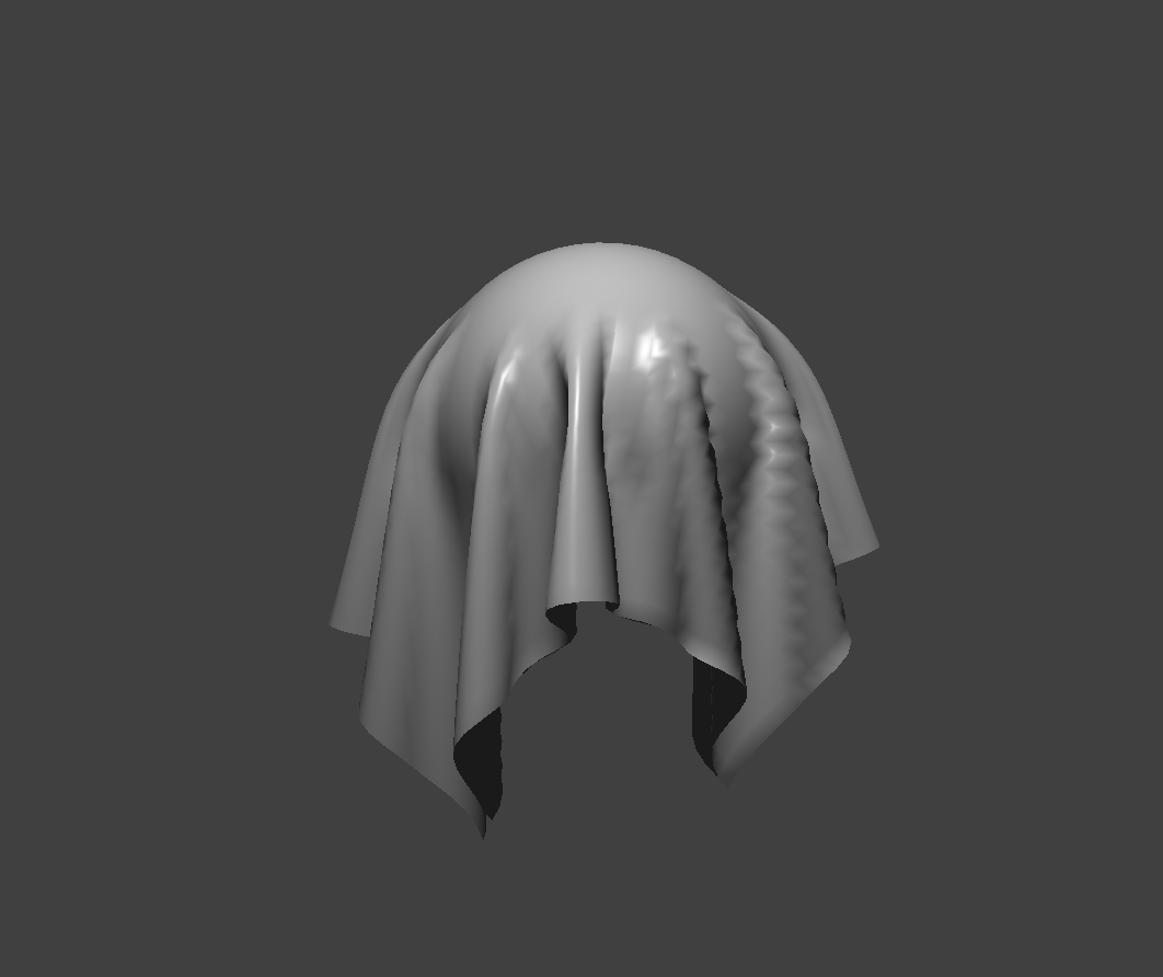
Here are the results of running the cloth collision test with a sphere. As we increase \(k_s\), the stretchiness factor of the cloth, we see that it maintains more of its shape and becomes more rigid.

Here is the cloth lying on a plane:

Self-Collisions

To prevent the cloth from folding over and intersecting with itself, we also need to handle self-collisions. The naive \(O(n^2)\) way of doing this would be to check if every mass is about to collide with every other mass in the grid at every time step, but this is too inefficient for real-time simulations.

Instead, I implement spatial hashing. I subdivide the entire space into the scene into equally sized 3D boxes, map each box to a unique float, and then build a hash table from each float to a list of point masses located in the box. Then, at every time step, I only need to build the hash table and iterate through the point masses. For each point mass, I use the hash table to find a list of neighboring point masses in the same 3D volume and check for collisions between each point mass and its neighbors.

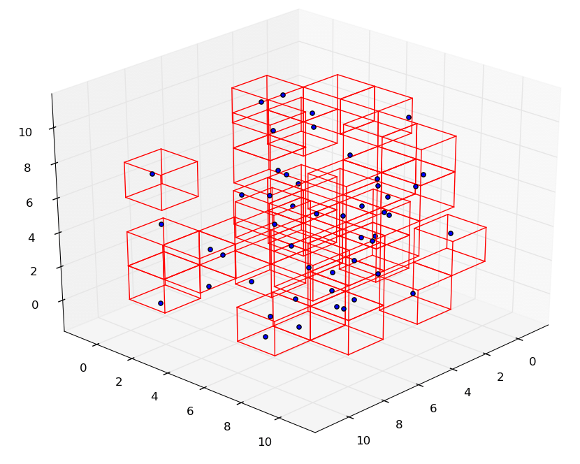
To map a 3D volume to a float, I take the coordinates of the box \((x, y, z)\) and return \(p^2x + py + z\), where \(p\) is a sufficiently large prime number. Because \(p\) is prime, \(p^2\), \(p\), and \(1\) are unlikely to have any linear combinations that produce the same value. A large enough prime creates a larger separation between \(p^2\), \(p\), and \(1\), which reduces the risk of collisions for large ranges of \((x, y, z)\).

To see if two point masses are about to collide, I check if they are 2 * cloth_thicknesses apart and apply a correction vector to ensure they are. The final correction vector applied to each point mass is the average of all correction vectors from its neighboring point masses, scaled down by the number of simulation steps to avoid too many sudden position corrections.

Below are the results of the cloth falling onto itself:

Note that as we increase the spring constant \(k_s\), the cloth folds upon itself fewer times because it simulates a stiffer fabric.

GLSL Shaders

Diffuse and Blinn-Phong Shading

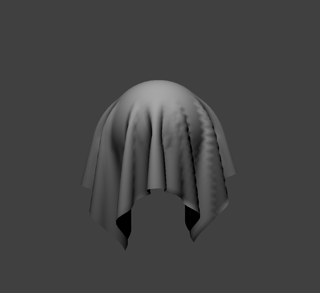
I first implement diffuse and Blinn-Phong shading using a default vertex shader and different fragment shaders. The default GLSL vertex shader takes in per-vertex model-space attributes in_position and in_normal and use the model-to-world space and world space-to-screen space matrices to output v_position and v_normal for the fragment shader.

The light intensity \(I\) and light position are provided as uniforms to the fragment shader, and we can find \(l\) (and \(r\)) by finding the vector from the light position to v_position. We set the alpha of the output color to 1 for diffuse shading.

Blinn-Phong shading is just like diffuse shading but with additional ambient light and specular light terms:

The Blinn-Phong fragment shader has the light position and camera position as uniforms, so we can find the incoming and outgoing light directions w_i and w_o. The vector \(h\) is the bisector between w_i and w_o.

Texture Mapping

The default vertex shader also provides the fragment shader with a UV coordinate to index into the texture uniform with the built-in GLSL function texture(sampler2D tex, vec2 uv). Now, we can apply pre-loaded textures to the cloth as well:

Displacement and Bump Mapping

We can also encode a height map in a texture to simulate changes in the surface of an object. With bump mapping, we can give the illusion of surface irregularities in height (bumps) by adjusting the normal vectors of an object.

Using a texture map as a height map, I find the local space normals by looking at how the height \(h(u,v)\) changes as we make small changes in \(u\) or \(v\). We can get \(h(u,v)\) from a texture in different ways, such as by taking the r channel or the norm of the rgb-vector.

To turn the local normal back into the model space normal, we can multiply by the tangent-bitangent-normal (TBN) matrix. The tangent vector can be pre-computed from the mesh geometry and loaded into the vertex shader, and passed into the fragment shader from there.

In displacement mapping, we also modify the positions \(p\) of the vertices in the vertex shader in the direction of the original model space vertex normal \(n\), scaled by a factor \(k_h\).

Now, we also observe a change in the geometry of the cloth:

Environment Reflection Mapping

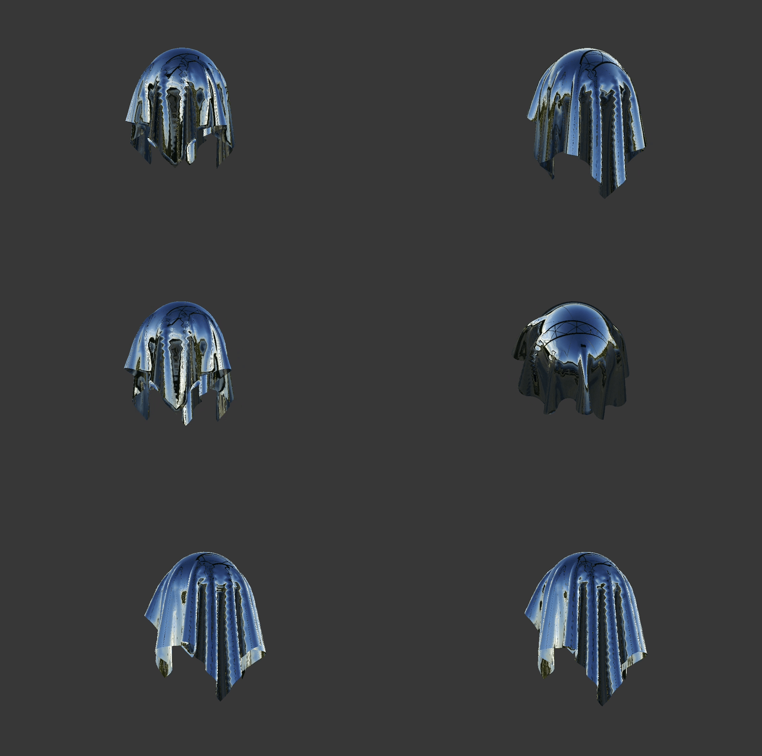
Using a pre-computed cubemap, we can sample from an environment texture using a 3D direction vector. To get envrionmental reflections on our cloth, we can compute the incoming light direction w_i by reflecting the outgoing eye-ray over the surface normal, and use that to sample a cubemap uniform with texture(samplerCube tex, vec3 dir). Below shows the result of the cloth with this mirror-like texture: